Theory reminder
Hypotheses
This section is just a short reminder about linear potential flow theory. Please refer to complete lectures for details.
Linear potential flow theory assumes
Potential flow (inviscid, incompressible and irrotational)
Small amplitude motions (body boundary condition linearized at the equilibrium position)
A small wave steepness (\(a/ \lambda \ll O(1)\)) and linearized free surface boundary conditions (at \(z=0\)).
It applies when the effect of flow separation on the hydrodynamic loads is limited (\(K_C < 2\))
Body motions
When the body is at its equilibrium position, its position is \(\vec{X}=0\). \(\vec{X}\) is the generalized position vector, with 6 elements, one for each degree of freedom of the system:
Loads acting on the body
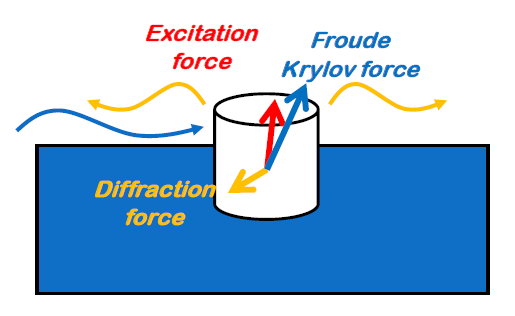
The hydrodynamic loads acting on the body are decomposed into the following categories (see Figure 2):
The excitation force \(\vec{F}_e\): forces and moments due to the waves. They can be decomposed into:
Froude-Krylov force \(\vec{F}_{FK}\) (unsteady pressure field of the undisturbed wave on the body geometry)
Diffraction force \(\vec{F}_d\) (diffracted wave pressure field on the body geometry)
Note
The excitation forces (Froude-Krylov and diffraction) are usually written for a unit wave amplitude. To find the actual force acting on the body, the excitation forces must be multiplied by the wave amplitude \(a\).
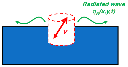
Radiation forces are induced by the waves created by the motions of the body. They can be further decomposed between added mass and damping:
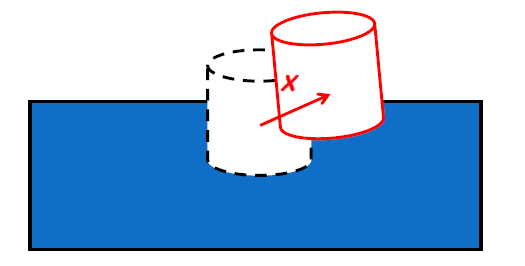 Small body motion
 Diffraction
 Radiation
Fig. 1 (Small) motions of a floating body and decomposition of the hydrodynamic forces
Eventually, we can also consider:
Hydrostatic force or buoyancy. For small motions, the hydrostatics acts as a linear stiffness with a stiffness K_h. K_h is a 6-by-6 matrix and the force is computed as:
The mooring forces can also be approximated as a linear stiffness if the motions amplitudes are sufficiently small:
Added damping from friction or other energy dissipation phenomena:
Boundary Elements Method (BEM) codes are usually employed to compute the hydrodynamic coefficients \(M_a\) and \(B_r\), as well as the excitation force Fe and the hydrostatic stiffness matrix \(K_h\). From these, the RAOs of the system can be found, which describe the behaviour of the system in waves.
Note
The hydrodynamic coefficients \(M_a\) and \(Br\) are sometimes written \(A\) and \(B\) respectively.
Response Amplitude Operator
The Response Amplitude Operator (RAO) is a frequency-domain representation of the system’s response to waves. It is defined as the ratio of the amplitude of the response to the amplitude of the wave, for a given frequency.
where \(X\) is the amplitude of the response and \(a\) is the amplitude of the wave.
Considering the previous expression of the hydrodynamic forces acting on the body, the RAO can be written as:
where \(M\) is the mass matrix of the body and the other symbols are as previously defined.
Impulse Response Functions
In order to find the hydrodynamic forces in the time domain, the Cummins-Ogilvie method can be used. This method is based on the computation of the impulse response functions (IRF) of the system. The IRF is the response of the system to an impulse force acting on the body. It is defined as:
where \(B_\infty\) is the asymptotic value of the radiation damping coefficient \(B_r(\omega)\) when \(\omega \rightarrow \infty\).
Note
The IRF is sometimes called the retardation function in the literature.
The radiation force can then be expressed in the time domain as:
where \(A\) is the asymptotic value of the added mass coefficient \(M_a(\omega)\) when \(\omega \rightarrow \infty\).
Note
For a body without forward velocity (as is the case in Nemoh), it can be proven that \(B_\infty = 0\), slightly simplifying the equations.
The excitation force can be computed in the time domain for each wave of frequency \(\omega\), direction \(\beta\) and amplitude \(a\) as: