Post-processing
The easiest way to visualize the results is to use Tecplot or any other software that can read the files generated by Nemoh with the tecplot format.
Most results are also output in a custom text format (.dat files).
Post-processing 2D data
The results are stored in the results directory. The main files are:
RadiationCoefficients.tec: added mass coefficients \(M_{a_{ij}}\) (also inCM.dat) and radiation damping coefficients \(B_{r_{ij}}\) (also inCA.dat)FKForce.tec: Froude-Krylov forces \(\vec{F}_{FK}\)DiffractionForce.tec: diffraction forces \(\vec{F}_d\)ExcitationForce.tec: excitation forces \(\vec{F}_e\)
Depending of the post-processing options, other files may be present in the results directory (such as Impulse Response Functions (IRF) and Response Amplitude Operators (RAO)).
Loading a file in Tecplot
To load a file in Tecplot, click on File -> Load Data... and select the file you want to load.
Alternatively, directly click the Load Data button on the top left.
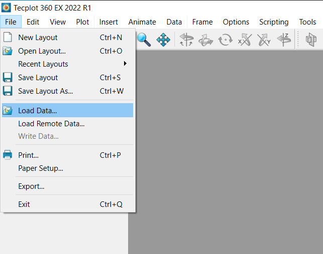
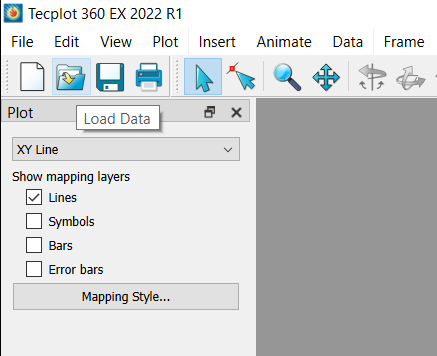
Fig. 3 Two ways of loading data in Tecplot
The file will be loaded in Tecplot and you can visualize the results in the main window.
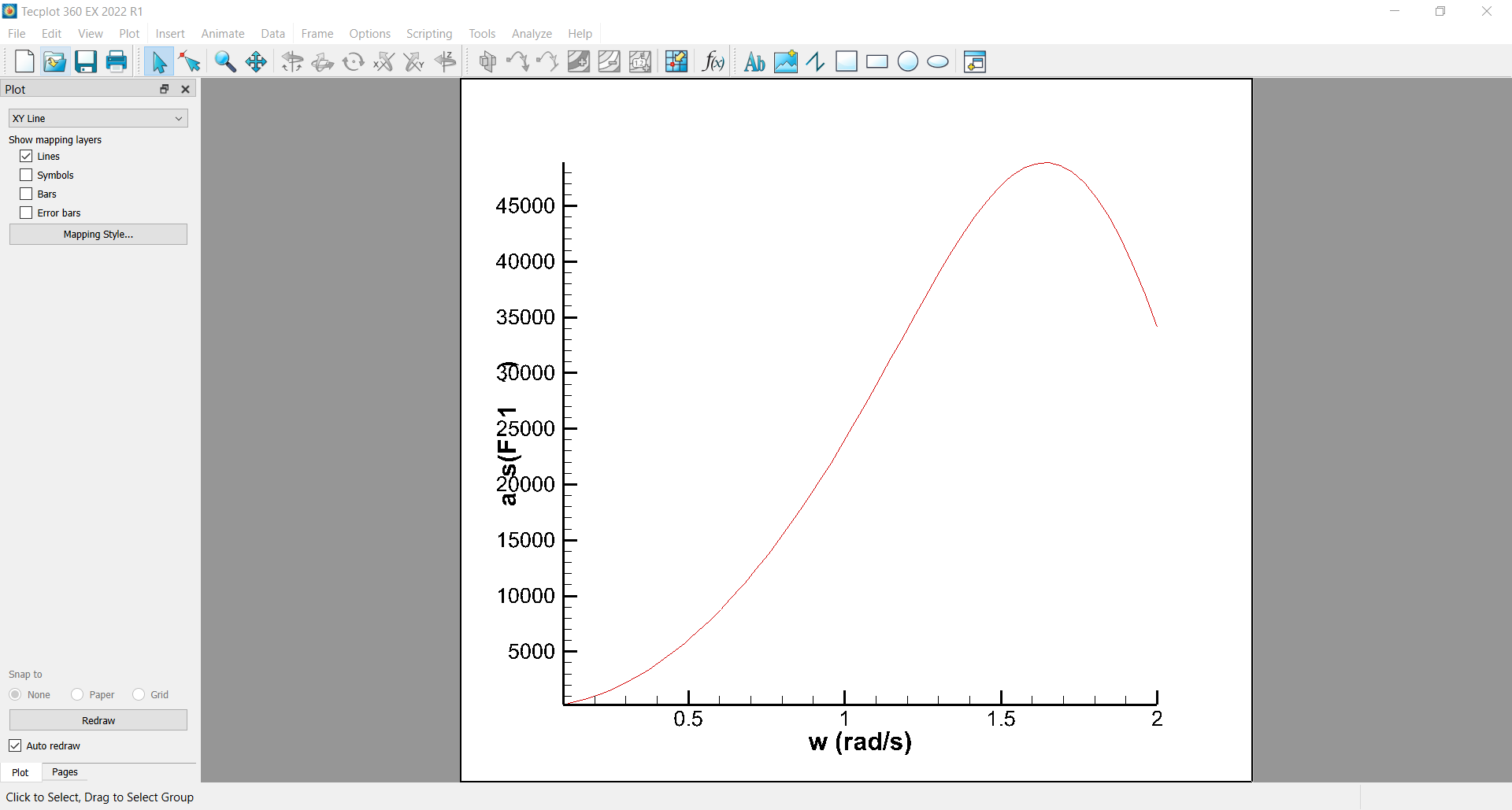
The Nemoh output files each contain data for all requested body Degrees of Freedom (DoF) and/or forces, as functions of the wave frequency. Some files also have data for different wave directions.
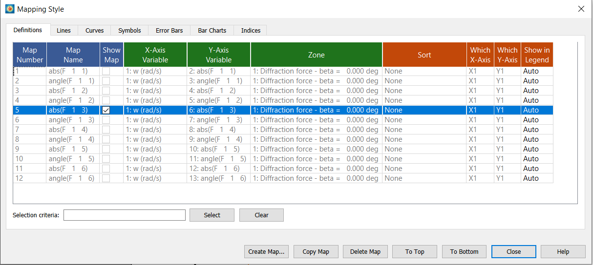
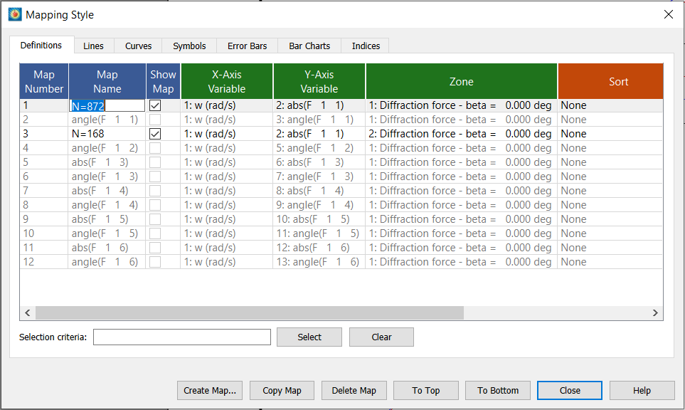
To select the data you want to display, click on the Mapping Style... button on the left.
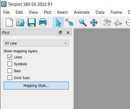
In the small window that appears, navigate to the Definitions tab and check the box in the Show Map column for the data you want to display.
You can check several curves to display them all on the same plot.
Hint
After changing the plotted data in the Mapping Style window, click on View -> Fit to Full Size (or hit Ctrl+F) to update the scales to the new data.
The other tabs in the Mapping Style... window allow you to customize the display of the data.
Hint
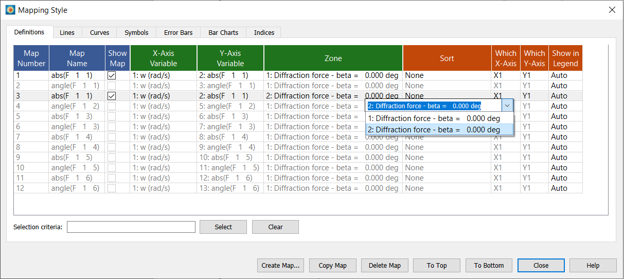
The Zone column allows you to switch between different wave directions.
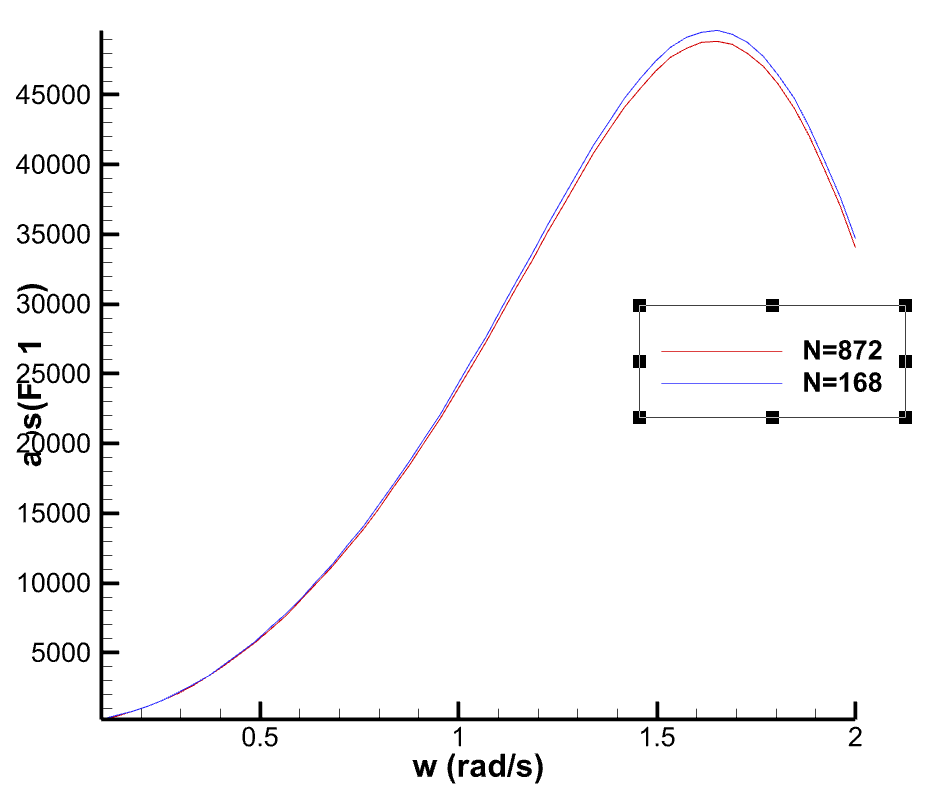
Comparing results from different files
To open other results for comparison, click on File -> Load Data... (or the Load Data button) again and select the file you want to load.
In the following prompt, select Append data to active frame to add the new data to the existing plot.
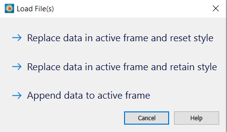
Warning
Appending data is trivial when the files contain the same data fields, as is most often the case when one wants to compare. However, if the files contain different data fields, Tecplot will prompt you to merge some fields and add others. This can be confusing and is not recommended.
A new Zone has been added, which can be selected in the Zone column in the Mapping Style window.
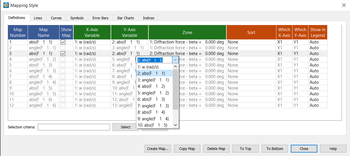
In order to compare the same data from different files, make sure that the relevant field is selected in the Y-Axis column.
Displaying a legend
To display a legend, click on Plot -> Line Legend... and check the Show Line Legend box (and the Show Mapping Names box).
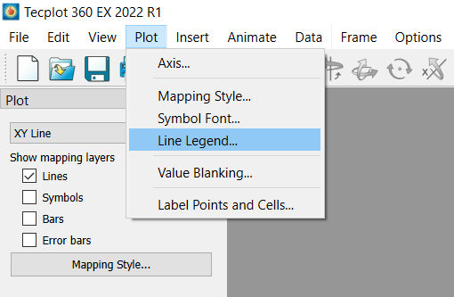
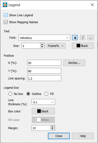
Fig. 4 Displaying the line legend
You can edit the names displayed in the legend in the Mapping Style window.
The legend will be displayed in the plot, and can be moved around by clicking and dragging it.
Post-processing 3D data
Two types of 3D data can be output by Nemoh (only if specicied in the Nemoh.cal file):
The pressure distribution on the body, in
pressure.<problem-number>.datfiles.The free surface elevation around the body, in
freesurface.<problem-number>.datfiles.
Hint
Keep in mind that Nemoh’s results are in the frequency domain. Thus, you won’t be able to see the waves as you could expect in the time domain. The displayed data is the amplitude or phase shift of a physical quantity.
Warning
Outputting the free surface elevation significantly increses the execution time of Nemoh.
To load a 3D file in Tecplot, click on File -> Load Data... and select the file you want to load (see last section).
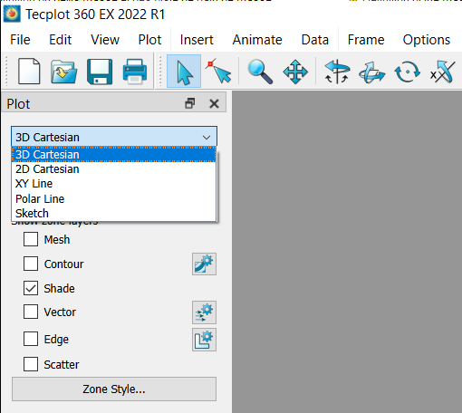
Instead of XY Line, select 3D cartesian in the dropdown menu on the left.
You can that select the type of data you want to display. Check the Mesh and Contour boxes to display the mesh and the surfacic data, respectively.
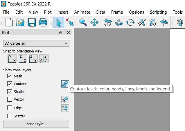
Click on the button next to Contour to select the surfacic fields you want to display.
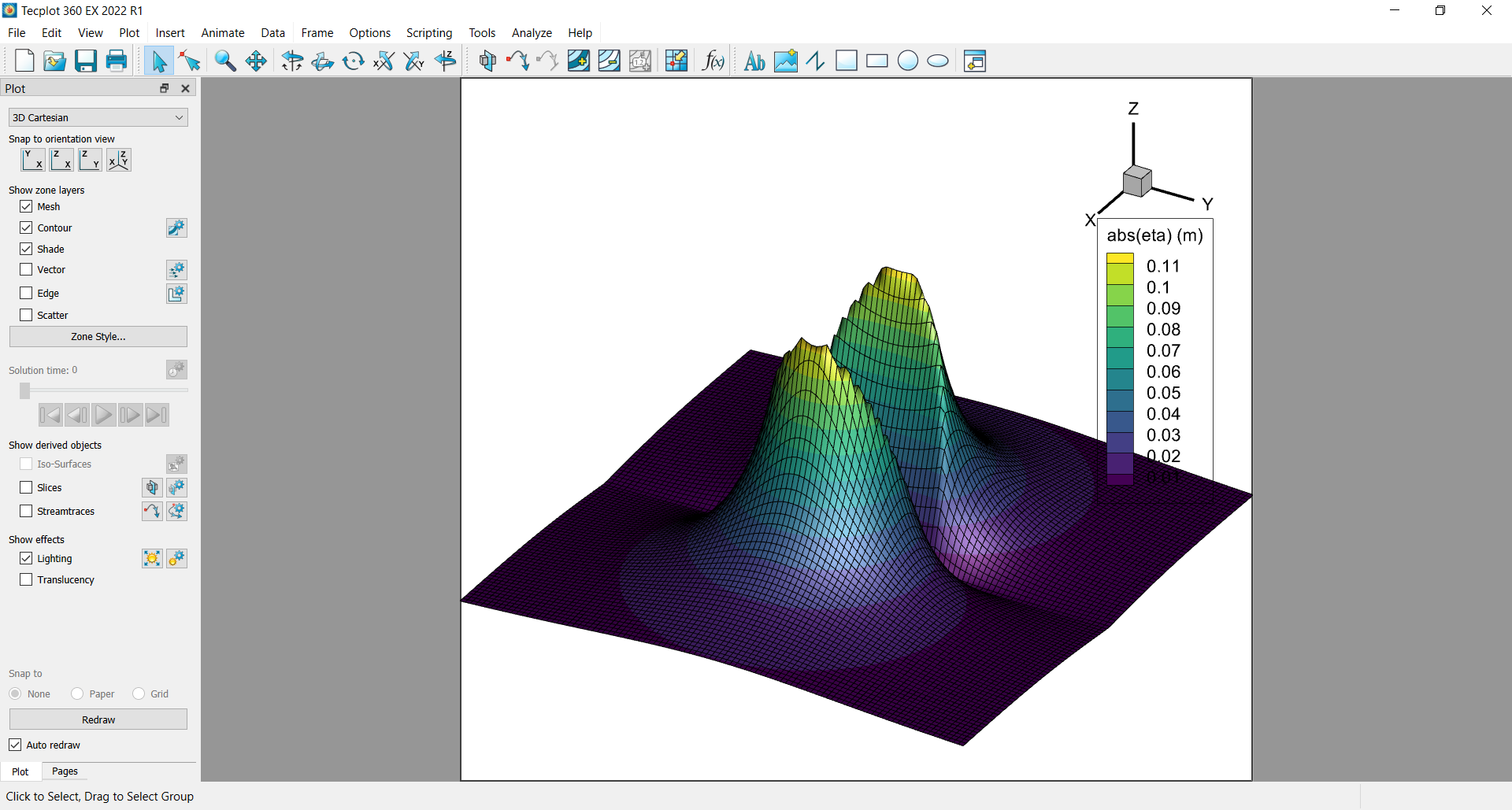
The surfacic data will be displayed on the mesh.
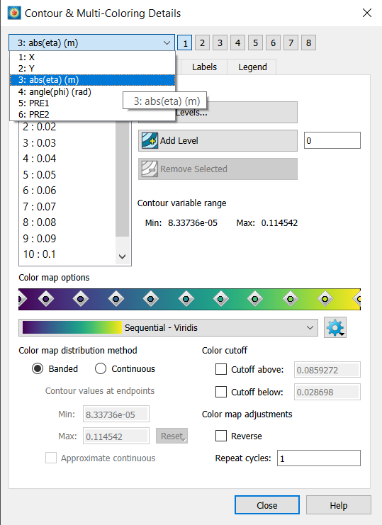
You can choose another colormap in the Contour options window. You can also choose a continuous colormap rather than a banded one.
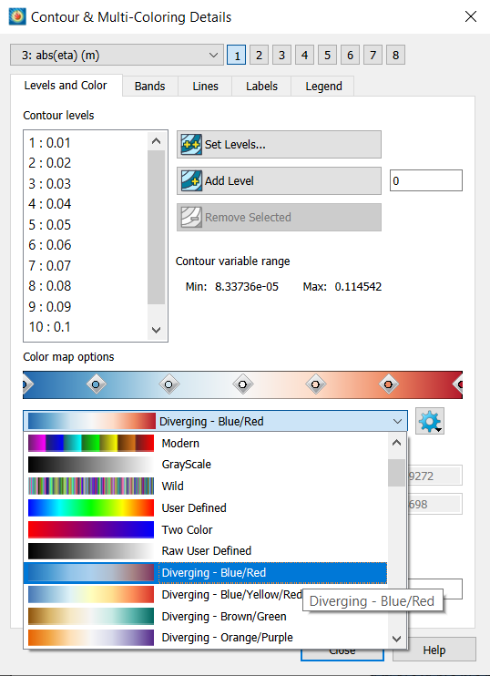
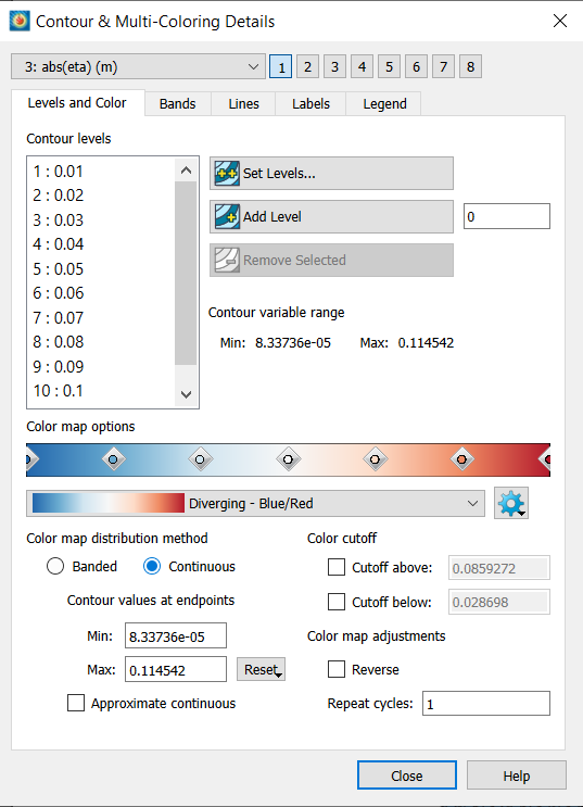
Fig. 5 Colormap options